Interpreting a learned policy
A learned policy is often treated as a black box, but for the applied environments its decision rule lives in a small, interpretable state space, so it can be drawn. This makes it possible to check what the agent learned, not just that its return went up.
The figure below trains a DQN on
NonstationaryInventory
and plots the order quantity it chooses at every state (inventory on hand against recent
demand), next to the two classical rules on the same grid. Reproduce it with:
python examples/policy_heatmap.py
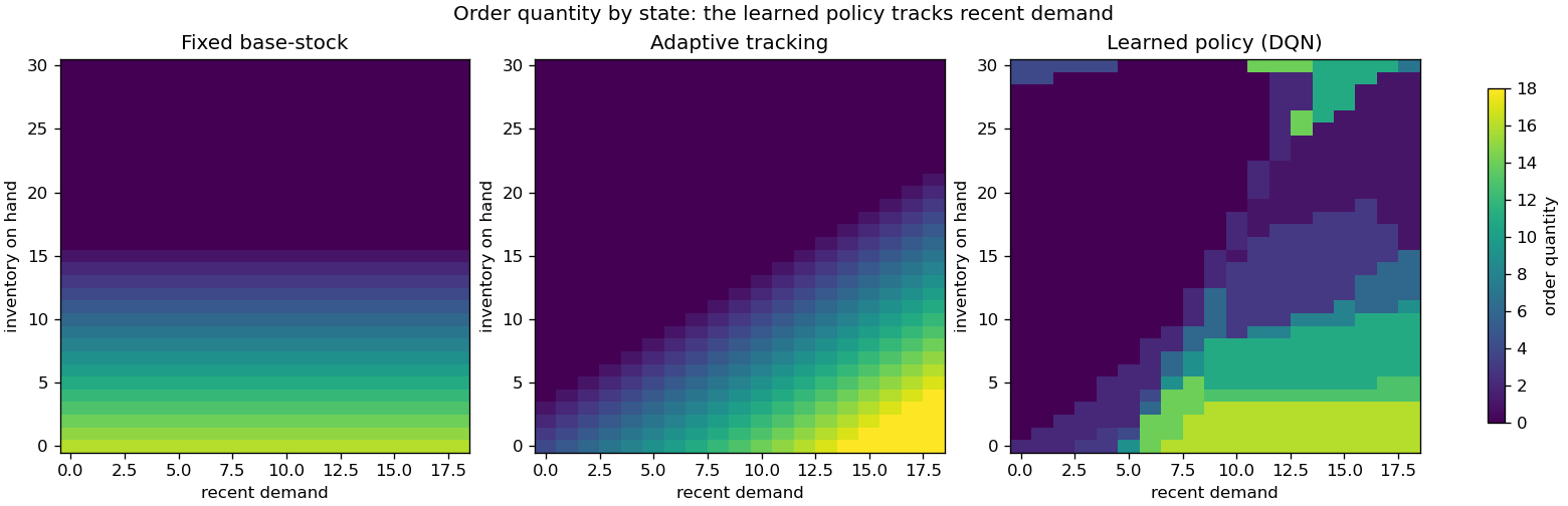
Reading the three panels:
- Fixed base-stock. The order depends only on inventory (horizontal bands) and ignores recent demand. This is the rule's defining limitation: one order-up-to level for every demand era.
- Adaptive tracking. The order rises with recent demand and falls with inventory, a clean diagonal structure. This is the rule that encodes the right domain knowledge.
- Learned policy. The DQN was given only the reward signal, yet its map resembles the adaptive rule far more than the fixed one: it too raises the order when recent demand is high. That is the mechanism behind its edge over the fixed base-stock, made visible.
The point is not that the learned policy is perfect (its map is noisier, and a hand-coded adaptive rule does better still, as the case study shows). It is that the policy is inspectable: you can see the structure it discovered and judge whether it is sensible before trusting it.